The vacuum is not empty. It is extremely busy.

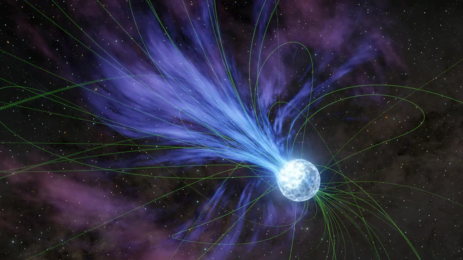
Empty space has energy, structure, and effects you can measure. The quantum vacuum splits the energy levels of hydrogen, pulls two uncharged mirrors together, and bends X-rays travelling out of a magnetar’s magnetosphere. It also produces the single worst prediction in physics, wrong by up to 120 orders of magnitude. Here is what is established, what is contested, and what nobody has solved.

Take a sealed box. Pump out every atom of gas. Cool the walls toward absolute zero so no thermal radiation leaks in. Shield it from every external field you can name. What remains is, by any reasonable definition, nothing.

It is not nothing. It is the quantum vacuum: the lowest-energy state a quantum field can occupy. That is a different statement from saying it is a state of zero energy, and the gap between those two ideas holds a surprising amount of twentieth-century physics.

Why the lowest-energy state is not a still one

Start with the simplest system in quantum mechanics: the harmonic oscillator.

Classically, an oscillator at rest has zero energy. Quantum mechanically it cannot. The uncertainty principle forbids fixing position and momentum at the same time, so a quantum oscillator in its ground state keeps an irreducible residue of energy, ½ℏω. It is not tracing a path back and forth. It is not sitting still either. That residue is zero-point energy, and it is not optional. Removing it would violate the uncertainty principle.

Quantum field theory applies that result everywhere at once. In QFT a field is an infinite collection of oscillators, one for every mode it can support, meaning every combination of momentum and polarisation. The vacuum is the state in which all of them sit in their ground states, and each contributes its own ½ℏω.

Two things follow. The vacuum acquires a nonzero energy density. The fields acquire nonzero variance. Measure the electromagnetic field at a point in empty space many times over and you will not get zero every time. You get a distribution centred on zero, with fluctuations around it.

That variance is the busy part. The vacuum is not a substance, and it is not full of tiny objects. It is not inert either.

What virtual particles actually are

Virtual particles are a calculational device, not a sequence of events.

The popular version says particle–antiparticle pairs constantly appear and vanish in empty space, borrowing energy from the uncertainty principle and repaying it before anyone notices. That description invites a specific wrong inference, so it is worth replacing.

Virtual particles are internal lines in Feynman diagrams. They are bookkeeping terms in a perturbative expansion used to compute interaction probabilities. They do not satisfy the relationship between energy, momentum and mass that real particles obey. Nothing detects them and no experiment counts them. Take a different computational route to the same physics, a lattice calculation for instance, and the virtual particles vanish from the mathematics while every prediction stays identical.

So the honest account runs like this. The vacuum has fluctuating fields. When we compute the consequences of those fluctuations perturbatively, virtual particles show up as intermediate terms. The fluctuations are physical. The particles are accounting, and they happen to be extremely effective accounting.

The Lamb shift

Vacuum fluctuations split two hydrogen levels that the Dirac equation says should be identical.

In 1947 Willis Lamb and Robert Retherford drove microwave transitions in a beam of excited hydrogen and found the 2S₁ᐟ₂ and 2P₁ᐟ₂ states separated by roughly 1,000 megahertz. The modern value is about 1,058 MHz. Dirac’s theory predicts exactly zero.

The splitting comes from the electron’s coupling to vacuum fluctuations of the electromagnetic field. Those fluctuations smear the electron’s position slightly, which changes how strongly it feels the proton’s charge. The 2S state carries more probability density at the nucleus, so it shifts further.

Hans Bethe produced a working estimate within weeks. The measurement is generally credited with forcing quantum electrodynamics into its modern renormalised form.

The electron’s magnetic moment

Dirac’s theory predicts the electron’s gyromagnetic ratio g should be exactly 2. It is not, and the excess is vacuum structure.

The best measurement comes from Gerald Gabrielse’s group at Northwestern, published in 2023. A single electron held in a trap for months gives g/2 = 1.001 159 652 180 59 (13), a fractional precision of 0.13 parts per trillion. It is the most precisely determined property of any elementary particle.

QED calculates that same excess from the electron’s interaction with fluctuating fields. Theory and experiment agree to about one part in 10¹².

One caveat deserves stating plainly. The Standard Model prediction is a function of the fine structure constant α, and independent determinations of α disagree with each other. That disagreement now limits the comparison, not the electron measurement. Settling it would sharpen the test by roughly an order of magnitude.

The Casimir effect

Two uncharged parallel plates in vacuum attract each other. Hendrik Casimir predicted it in 1948.

Plates placed very close together restrict which electromagnetic modes can exist in the gap, because only wavelengths that fit are allowed. The region outside supports the full spectrum. That imbalance in vacuum fluctuation pressure pushes the plates together.

The force is tiny and falls off sharply with separation, so a convincing measurement waited until 1997. Steve Lamoreaux mapped it across separations of 0.6 to 6 micrometres and found agreement with theory at roughly the 5 percent level. Many groups have measured it since.

At nanometre scales it stops being a curiosity. Casimir attraction is a live engineering constraint in micro-electromechanical devices, where it makes moving parts stick to their neighbours.

Running couplings

The strength of the electromagnetic interaction is not a fixed number. It grows at higher energy, which is to say at shorter distance. The fine structure constant is about 1/137 at low energy and about 1/128 at the mass of the Z boson, near 91 GeV.

The standard interpretation is vacuum polarisation. A bare charge polarises the vacuum around it, and that polarised vacuum screens the charge. Probing more closely means penetrating the screen and seeing more of what sits underneath.

Quantum chromodynamics runs the other way. Gluons carry colour charge and interact with each other, which anti-screens instead of screening, and the result is asymptotic freedom. Quarks behave almost as free particles at high energy and cannot be pulled apart at low energy. Colliders including the LHC have tracked this running across several orders of magnitude in energy, and quantum processors have now watched confinement unfold in real time in simplified gauge theories.

Vacuum birefringence has resisted the laboratory for ninety years

In 1936 Werner Heisenberg and Hans Euler showed that a strong enough magnetic field should make the vacuum birefringent. Light polarised parallel to the field would travel at a very slightly different speed from light polarised perpendicular to it. Classical electromagnetism forbids this, since the vacuum offers no medium to do the refracting. In QED the field couples to vacuum fluctuations and empty space acquires an effective optical property.

The obstacle is scale. The effect only becomes appreciable near the Schwinger critical field, about 4.4 × 10⁹ tesla. The strongest continuous laboratory magnets reach roughly 45 tesla, a hundred million times short.

PVLAS chased it anyway, from 1993 onward, using a high-finesse optical cavity and rotating 2.5 tesla permanent magnets. Its final result gives a refractive index difference of (12 ± 17) × 10⁻²³, consistent with zero. QED predicts 2.5 × 10⁻²³ at that field strength, so after 25 years the experiment’s uncertainty still sat about a factor of seven above the signal it was built to find. No laboratory has detected vacuum birefringence.

The strongest evidence comes from a magnetar

Magnetars carry surface fields above 10¹⁴ gauss, which is 10¹⁰ tesla. No experiment reaches those conditions, so the test moved to the sky.

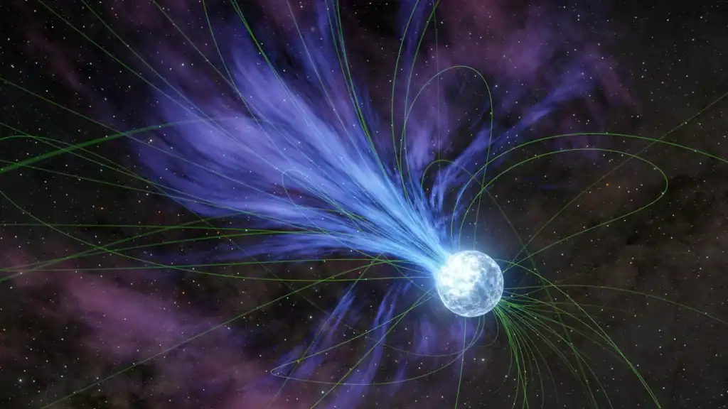
A team led by Rachael Stewart published phase- and energy-resolved X-ray polarisation measurements of the radio magnetar 1E 1547.0−5408 in Nature in August 2026. The observations combined the Imaging X-ray Polarimetry Explorer (IXPE) with NICER and radio data from Parkes/Murriyang.

The numbers: polarisation degree reaches 65 percent phase-averaged at 2 keV in the thermally dominated soft band, then drops substantially between 2 and 4 keV. At certain rotational phases the 2 to 3 keV polarisation climbs to nearly 80 percent, and it stays above about 40 percent throughout the radio beam crossing. Both the X-ray and radio polarisation angles follow the rotating vector model, which indicates the emission geometry tracks the star’s large-scale field.

The part nobody has solved

Everything above is a success story. Here is the failure.

If the vacuum has an energy density, that energy should gravitate. General relativity does not care what form energy takes. It curves spacetime regardless. So vacuum energy density should appear in Einstein’s equations as a cosmological constant, driving cosmic expansion.

We have measured that expansion since 1998. We can also calculate what quantum field theory predicts for the vacuum energy density. The two numbers do not agree. Depending on where you cut off the sum over modes, at the Planck scale or the electroweak scale or somewhere else, the theoretical value exceeds the observed one by something between sixty and a hundred and twenty orders of magnitude.

This is not a small discrepancy needing a correction factor. Candidate explanations include supersymmetric cancellations between bosonic and fermionic contributions, anthropic selection across a landscape of vacua, and the possibility that the calculation asks the wrong question because we lack a working theory of quantum gravity. None of them is established.

The problem sits at the intersection of our two most successful theories, and it says at least one of them is incomplete in a way we do not yet understand.

The vacuum decides what has mass

There is a practical reason to keep the vacuum in view. The Higgs mechanism works precisely because the vacuum is not empty in the naive sense.

The Higgs field holds a nonzero value everywhere, around 246 GeV, and particles acquire mass through their interaction with that background. The vacuum has a field configuration, and the properties of the matter we are made of follow from it.

Whether that configuration is stable remains open. Stability depends on the shape of the Higgs potential, which depends on the Higgs self-coupling, a number nobody has measured. It is the headline target of the High-Luminosity LHC upgrade now underway at CERN.

Which is a fair summary of where the subject stands. We can calculate the vacuum’s consequences to twelve digits and confirm them in a trap. We can watch it reshape X-rays leaving a neutron star. And we cannot say whether the vacuum we live in is the final one or a metastable state with a very long lifetime.

References

• W. E. Lamb & R. C. Retherford, Fine Structure of the Hydrogen Atom by a Microwave Method, Phys. Rev. 72, 241 (1947); DOI 10.1103/PhysRev.72.241
• X. Fan, T. G. Myers, B. A. D. Sukra & G. Gabrielse, Measurement of the Electron Magnetic Moment, Phys. Rev. Lett. 130, 071801 (2023); DOI 10.1103/PhysRevLett.130.071801; preprint arXiv:2209.13084
• H. B. G. Casimir, On the attraction between two perfectly conducting plates, Proc. K. Ned. Akad. Wet. 51, 793 (1948)
• S. K. Lamoreaux, Demonstration of the Casimir Force in the 0.6 to 6 μm Range, Phys. Rev. Lett. 78, 5 (1997); DOI 10.1103/PhysRevLett.78.5
• W. Heisenberg & H. Euler, Folgerungen aus der Diracschen Theorie des Positrons, Z. Phys. 98, 714 (1936); DOI 10.1007/BF01343663; English translation arXiv:physics/0605038
• A. Ejlli et al. (PVLAS), The PVLAS experiment: A 25 year effort to measure vacuum magnetic birefringence, Phys. Rep. 871, 1 (2020); preprint arXiv:2005.12913
• R. E. Stewart et al., Vacuum birefringence and the polarized X-ray emission from a radio magnetar, Nature (2026); DOI 10.1038/s41586-026-10859-z; preprint arXiv:2509.19446
• S. Weinberg, The cosmological constant problem, Rev. Mod. Phys. 61, 1 (1989); DOI 10.1103/RevModPhys.61.1